2D FEA Validation
This section details the validation for the 2D FEA calculator. Several examples are worked through to determine expected results such as deflections, forces, and stresses. These expected results are then compared to the actual output of the 2D FEA.
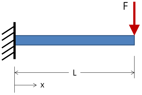
Cantilever Beam, End Load
The standard beam equations for a cantilever beam loaded at the free end are given below:
| Max Deflection: | $$ \delta_{max} = {P L^3 \over 3EI} $$ | @ x = L |
| Max Slope: | $$ \theta_{max} = {P L^2 \over 2EI} $$ | @ x = L |
| Shear: | $$ V = +F $$ | constant |
| Moment: | $$ M_{max} = -FL $$ | @ x = 0 |
For the validation case, an Aluminum 6061-T6 beam with a 1 inch diameter circular cross-section and a length of 10 inches will be loaded at 1000 lbf. The inputs are:
For the given inputs, the expected results are:
| Max Deflection: | \( \delta_{max} = 0.679 \text{ in} \) | @ x = L |
| Max Slope: | \( \theta_{max} = 0.1019 \text{ rad} \) | @ x = L |
| Shear: | \( V = +1000 \text{ lbf} \) | constant |
| Moment: | \( M_{max} = -10,000 \text{ in-lbf} \) | @ x = 0 |
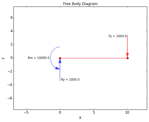
The Free Body Diagram (FBD) is shown below. From the FBD it can be seen that the forces balance and the beam is in static equilibrium.
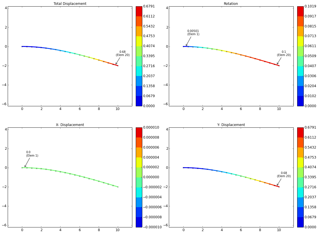
The displacement plots are shown below. From these plots it can be seen that a maximum displacement of 0.679 inches occurs at the free end of the beam as well as a maximum slope of 0.1019 radians.
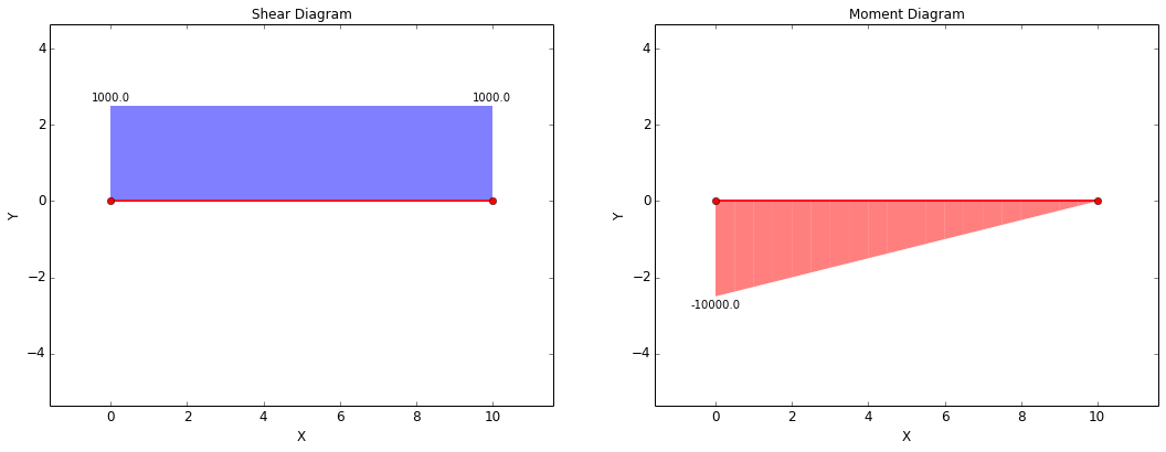
The shear-moment diagram for the beam is shown below. This diagram is what would be expected for the current case. A constant shear force of 1000 lbf exists along the length of the beam, and the moment increases linearly from 0 in-lbf at the free end of the beam to the full value of -10,000 in-lbf at the fixed end.
There are two points of interest for validating stresses. Before calculating stress, the forces at these points need to be determined.
| Axial (lbf) | Shear (lbf) | Moment (in-lbf) | |
|---|---|---|---|
| Forces @ x = 0: | $$ F_{ax} = 0 $$ | $$ F_{sh} = 1000 $$ | $$ M = 10000 $$ |
| Forces @ x = L: | $$ F_{ax} = 0 $$ | $$ F_{sh} = 1000 $$ | $$ M = 0 $$ |
The stresses are calculated using the following equations:
| Axial Stress | Shear Stress | Bending Stress | Von Mises Stress |
|---|---|---|---|
| $$ \sigma_{ax} = {F_{ax} \over A} $$ | $$ \tau_{sh} = {F_{sh} \over A} $$ | $$ \sigma_{b} = {Mc \over I} $$ | $$ \sigma_{vm} = \sqrt{ (\sigma_{ax} + \sigma_{b})^2 + 3\tau_{sh}^2 } $$ |
Based on the forces at each point and the equations above, the expected stresses at the points of interest are:
| Tensile (psi) | Shear (psi) | Bending (psi) | Von Mises (psi) | |
|---|---|---|---|---|
| Stress @ x = 0: | $$ \sigma_{ax} = 0 $$ | $$ \tau_{sh} = 1273 $$ | $$ \sigma_{b} = 101859 $$ | $$ \sigma_{vm} = 101883 $$ |
| Stress @ x = L: | $$ \sigma_{ax} = 0 $$ | $$ \tau_{sh} = 1273 $$ | $$ \sigma_{b} = 0 $$ | $$ \sigma_{vm} = 2205 $$ |
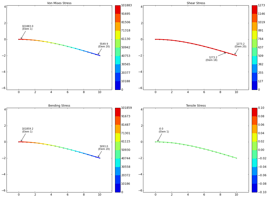
The stress plots are shown below. It can be seen that these plots agree with the stresses calculated above.
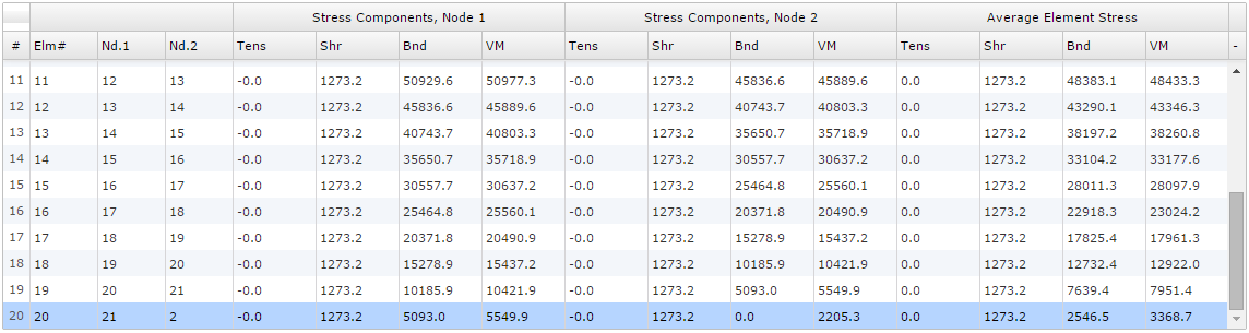
There is one discrepancy that can be noted, which is that the values for bending stress and von Mises stress at x = L are shown to be higher in the stress plots than predicted. The reason for this is that the stress plots are showing the maximum nodal values for each element, and the maximum bending stress for the element at x = L will occur at the left-most node in that element. Therefore, the values of bending stress and von Mises stress reported in the plots will be somewhat higher than what was calculated above. However, the stresses for each node within any element can be interrogated in the result tables. This table will be discussed following the stress plots.
A screenshot of one of the result tables for this case is shown below with the element of interest highlighted. The node at the very end of the beam (i.e. at x = L) is "Node 2" for the highlighted element. It can be seen that the bending stress at this node is 0 psi and the von Mises stress at this node is 2205.3 psi. This matches what was predicted.