


Fracture Mechanics
Contents
Overview
Fracture mechanics is a methodology that is used to predict and diagnose failure of a part with an existing crack or flaw. The presence of a crack in a part magnifies the stress in the vicinity of the crack and may result in failure prior to that predicted using traditional strength-of-materials methods.
The traditional approach to the design and analysis of a part is to use strength-of-materials concepts. In this case, the stresses due to applied loading are calculated. Failure is determined to occur once the applied stress exceeds the material's strength (either yield strength or ultimate strength, depending on the criteria for failure).
In fracture mechanics, a stress intensity factor is calculated as a function of applied stress, crack size, and part geometry. Failure occurs once the stress intensity factor exceeds the material's fracture toughness. At this point the crack will grow in a rapid and unstable manner until fracture.

Fracture mechanics is important to consider for several important reasons:
- Cracks and crack-like flaws occur much more frequently than might be expected. Cracks can either pre-exist in a part, or they can develop due to high stress or fatigue.
- Typically, as the strength of a material increases, fracture toughness decreases. The intuition of many engineers to prefer higher strength materials can lead them down a dangerous path.
- Ignoring fracture mechanics can lead to failure of parts at loads below what is expected using a strength-of-materials approach.
- A failure due to brittle fracture is rapid and catastrophic and provides little warning.
The image below shows the SS Schenectady tanker, one of the World War II Liberty Ships and one of the most iconic fracture failures. The Liberty ships all had a tendency to crack during cold weather and rough seas, and multiple ships were lost. Approximately half of the cracks initiated at the corners of the square hatch covers which acted as stress risers. The SS Schenectady split in two while sitting at dock. An understanding of fracture mechanics would have prevented these losses.

Stress Concentrations Around Cracks
Cracks act as stress risers and cause the stress in the part to spike near the tip of the crack. As a simple example, consider the case of an elliptical crack in the center of an infinite plate:

The theoretical value of stress at the tip of the ellipse is given by:

where σ is the nominal stress and ρ is the radius of curvature of the ellipse, ρ = b2/a.
As the radius of the crack tip approaches zero, the theoretical stress approaches infinity. This infinite stress is known as a stress singularity and is not physically possible. Instead, the stress distributes over the surrounding material, resulting in plastic deformation in the material at some distance from the crack tip. This region of plastic deformation is called the plastic zone and is discussed in a later section. The plastic deformation causes blunting of the crack tip which increases the radius of curvature and brings the stresses back to finite levels.
Because of the stress singularity issues that arise when using the stress concentration approach, and because of the plastic zone that develops around the crack tip which renders the stress concentration approach invalid, other methods have been developed for characterizing the stresses near the tip of the crack. The most prevalent method in use today is to calculate a stress intensity factor, as discussed in a later section.
Looking for Fracture Calculators?
We have a few to choose from:

Modes of Loading
There are three primary modes that define the orientation of a crack relative to the loading. A crack can be loaded in one mode exclusively, or it can be loaded in some combination of modes.

The figure above shows the three primary modes of crack loading. Mode I is called the opening mode and involves a tensile stress pulling the crack faces apart. Mode II is the sliding mode and involves a shear stress sliding the crack faces in the direction parallel to the primary crack dimension. Mode III is the tearing mode and involves a shear stress sliding the crack faces in the direction perpendicular to the primary crack dimension.
Engineering analysis almost exclusively considers Mode I because it is the worst-case situation and is also the most common. Cracks typically grow in Mode I, but in the case that the crack does not start in Mode I it will turn itself to become Mode I, as illustrated in the figure below.

Stress Intensity Factor
The stress intensity factor is a useful concept for characterizing the stress field near the crack tip.
For Mode I loading, the linear-elastic stresses in the direction of applied loading near an ideally sharp crack tip can be calculated as a function of the location with respect to the crack tip expressed in polar coordinates:


A term K, called the stress intensity factor, can be defined in the form:

where the units are either ksi√in or MPa√m.
The stress intensity factor for a Mode I crack is written as K I. (From this point forward, it is assumed that all stress intensity factors are Mode I for reasons discussed previously, so the stress intensity will be denoted simply as K. Using the equation for the stress intensity factor, the original equation for stress near the ideally sharp crack tip can be re-written as:

For θ = 0, the equation above simplifies to:

To extend the case of an ideally sharp crack tip to situations with real crack geometries, the stress intensity factor can be generalized as:

where a is the crack size and Y is a dimensionless geometry factor that is dependent on the geometry of the crack, the geometry of the part, and the loading configuration.
It is important to note that because equations describing the linear-elastic stress field were used to develop the stress intensity factor relationship above, the concept of the stress intensity factor is only valid if the region of plastic deformation near the crack tip is small. This will be discussed in more detail in a later section.
Stress Intensity Factor Solutions
The difficult part of calculating the stress intensity factor for a specific situation is finding the appropriate value of the dimensionless geometry factor, Y. This geometry factor is dependent on the geometry of the crack, the geometry of the part, and the loading configuration. A classic case is plate with a crack through the center, as shown below:

The stress intensity factor for a specific situation can be found through numerical methods such as Finite Element Analysis (FEA). However, solutions for many cases can be found in the literature. Solutions for some common cases, including the case shown above, can be found on our Stress Intensity Factor Solutions page.
Superposition for Combined Loading
Because the concept of the stress intensity factor assumes linear elastic material behavior, the stress intensity factor solutions can be combined by superposition to find solutions to more complex problems. For example, the stress intensity factor solution for a single edge cracked plate in tension can be combined with the solution for a single edge cracked plate in bending, as shown in the figure below.

The stress intensity factor for the combined solution is calculated as:

where σt is the applied tensile stress, σb is the applied bending stress, Yt is the geometry factor for the plate in tension, Yb is the geometry factor for the plate in bending, and a is the crack length.
Looking for Fracture Calculators?
We have a few to choose from:
Fracture Toughness
A material can resist applied stress intensity up to a certain critical value above which the crack will grow in an unstable manner and failure will occur. This critical stress intensity is the fracture toughness of the material. The fracture toughness of a material is dependent on many factors including environmental temperature, environmental composition (e.g., air, fresh water, salt water, etc.), loading rate, material thickness, material processing, and crack orientation to grain direction. It is important to keep these factors in mind when selecting a fracture toughness value to assume during design and analysis.
Fracture toughness values for many common engineering materials can be found in our database.
Fracture Toughness vs. Thickness
Fracture toughness decreases as material thickness increases until the part is thick enough to be in a plane-strain condition. Above this plane-strain thickness, the fracture toughness is a constant value known as the plane-strain fracture toughness. The plane-strain fracture toughness in Mode I loading is of primary interest, and this value is denoted by K IC.
The fracture toughness for a material at a specific thickness can be approximated as:

where t is the material thickness, Ak and Bk are material constants, and t0 is the plane-strain thickness at critical loading as calculated by:

where Sty is the tensile yield strength of the material.
The plot below was constructed using the thickness-specific fracture toughness equation above for an example material, 15-5PH, H1025. It can be seen that at lower thickness values the fracture toughness for this material is 90 ksi*in0.5, and the toughness drops to the plane-strain toughness value of 60 ksi*in0.5 as the thickness increases, after which the fracture toughness remains constant.

Even though the fracture toughness can be approximated as a function of the thickness of the part, it is still a good idea to use the plane-strain fracture toughness value in design and analysis.
Fracture Toughness vs. Strength
In general, within a specific class of materials, fracture toughness decreases as strength increases. If you start with a block of material and heat treat it and work it to increase the strength properties, you will also typically reduce the fracture toughness of the material.
The figure below shows fracture toughness vs. material strength for various classes of materials. It can be seen that for many materials, particularly for the engineering metal alloys and the engineering polymers, fracture toughness decreases with increasing strength.

Fracture Toughness vs. Crack Orientation
The fracture toughness of a material typically varies as a function of the crack orientation with respect to the grain direction. Because of this, fracture toughness values are typically reported along with the crack orientation.
The possible combinations of crack orientation and grain direction are shown in the figure below for both a rectangular shape and a cylindrical shape. Two-digit codes are used to denote the crack orientation. The first digit indicates the direction normal to the crack face. The second digit indicates the direction of the crack path.


Initial Crack Size
Cracks and crack-like flaws are common in engineering materials. Cracks will typically form around pre-existing flaws which act as stress concentrations and which, upon high stress or fatigue, develop into full-fledged cracks. Many flaws are serious enough that they should be treated as cracks, and these include deep scratches, inclusions of foreign particles, and grain boundaries. In addition to material flaws, geometric features in a part which act as stress concentrations can lead to crack initiation, including notches, holes, grooves, and threads. Cracks can also initiate from flaws introduced through other failure mechanisms, such as from pitting due to corrosion or from abrasion due to galling.
Determining the initial size of the crack is critical to assessing the potential for fracture. A conservative approach is to select a non-destructive evaluation (NDE) method for inspecting the part under consideration, and then to assume that a crack equal in size to the minimum detectable flaw size exists in the part in the most highly stressed location.
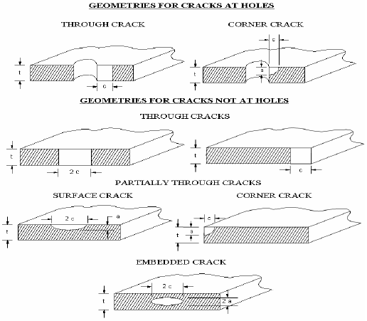
Many references are available that provide minimum detectable flaw sizes for various NDE methods, one of which is NASA-STD-5009. A table from NASA-STD-5009 is shown below for US units, along with a corresponding figure that provides the definitions of the crack dimensions "a" and "c".

If the minimum detectable flaw size is unknown, or if an NDE inspection is not planned for the part, then an alternate approach is to determine the critical crack size at the most highly stressed location in the part. If this critical crack size is very small, then it would be wise to inspect the part using an NDE method capable of detecting a crack of this size.
Looking for Fracture Calculators?
We have a few to choose from:
Plastic Zone Size
Plane-Stress vs. Plane-Strain
The size of the plastic zone is dependent on whether the part is considered to be in a plane-stress or a plane-strain condition. In plane-stress, the section is thin enough that the stresses through the thickness of the section are approximately constant. In plane-strain, stresses develop through the thickness of the section to resist contraction of the material and to keep the strain throughout the thickness approximately constant.
The part can be considered to be in plane-strain if the thickness satisfies the following condition:

where Kapp is the stress intensity at the applied stress and Sty is the material's tensile yield strength.
If the part thickness is less than that specified in the equation above, then the plastic zone size should be calculated assuming that the part is in plane-stress. The table below summarizes the plastic zone sizes for plane-stress and plane-strain.
| Plastic zone size for plane-stress: |

|
| Plastic zone size for plane-strain: |

|
The following sections provide more details on the derivation of the plastic zone size.
Plastic Zone Size for Plane-Stress
Due to the sharp nature of the crack, there will always be a plastic zone just ahead of the crack tip. We can use the elastic stress field equations (discussed in a previous section) to solve for the theoretical distance from the crack tip at which the stresses are equal to the material's yield strength. The elastic stress field equation is:

Setting the stress equal to the material's yield strength and solving for r gives the theoretical size of the plastic zone, rt:

where Kapp is the stress intensity due to applied stress, and Sty is the material's tensile yield strength.
For the actual plastic zone size to be equal to the theoretical plastic zone size, the stresses in the plastic zone must substantially exceed the material's yield strength. Because the yielded material in the plastic zone cannot support stresses much above the yield stress, the stresses near the crack tip are redistributed to the material farther out, and therefore the true size of the plastic zone is larger than the theoretical predicted value. The actual size of the plastic zone is approximately equal to 2rt, so a more realistic estimate of the plastic zone size, rp, is given by:

The figure below illustrates the theoretical elastic stress and plastic zone size, as well as the redistributed stresses and the resulting realistic estimate of the plastic zone size.

Note that the plastic zone size is proportional to (Kapp/Sty)2. This indicates that the plastic zone will be smaller for higher strength materials. Additionally, higher toughness materials are able to develop higher stress intensities before fracture, so the plastic zone will grow larger in higher toughness materials before failure occurs. Materials with low tensile strength and high fracture toughness can develop very large plastic zones at the crack tip.
Plastic Zone Size for Plane-Strain
The plastic zone size estimates described in the previous section apply to the plane-stress condition where the section is thin enough that the stresses through the thickness of the section are approximately constant. If the section is thick enough to be considered in plane-strain (i.e., stresses develop through the thickness of the section to resist contraction of the material and to keep the strain throughout the thickness approximately constant), then the size of the plastic zone is reduced as compared to that in the plane-stress condition.
The plastic zone size for the plane-strain condition can be approximated as:

where Kapp is the stress intensity due to applied stress, and Sty is the material's tensile yield strength.
Ductile vs. Brittle Fracture
There are two frames of reference when discussing ductile fracture versus brittle fracture. These frames of reference are the fracture mechanism and the fracture mode.
When materials scientists talk about brittle fracture and ductile fracture, they are typically referring to the fracture mechanism, which describes the fracture event at a microscopic level. In general, the brittle fracture mechanism is cleavage, and the ductile fracture mechanism is dimpled rupture, also known as microvoid coalescence. The cleavage mechanism is associated with brittle fracture. It involves little plastic deformation, and the fracture surface looks smooth with ridges. The microvoid coalescence mechanism is associated with ductile fracture. This mechanism involves the formation, growth, and joining of small voids in the material which is enabled through plastic flow, and the fracture surface looks dimpled like a golf ball.
When mechanical engineers talk about brittle fracture and ductile fracture, they are typically referring to the fracture mode, which describes the high-level behavior of the material during the fracture event. The figure below illustrates the fracture mode.

A load-displacement curve is shown along with cracked specimens placed at various locations along the curve. In the linear region of the curve with lower applied load, the stresses in the part are below the material yield strength. If the part were to fail in this region, this would be referred to as brittle fracture since the part has failed prior to what is predicted using strength-of-materials methods. Note that in this region, the plastic zone around the crack tip (shown in red) will typically be small, and so the linear elastic assumption applies and Linear Elastic Fracture Mechanics (LEFM) can be used to analyze the part. As the load increases, the plastic zone size increases. If the part fails in the higher region of the load-displacement curve, this is referred to as ductile fracture. If the plastic zone size has exceeded the applicability of LEFM but has not yet extended across the entire section, then elastic-plastic methods such as the Failure Assessment Diagram (FAD) can be used to analyze the part. Once the plastic zone size has extended across the entire section (gross section yielding), fracture mechanics methods can no longer be used, and the section will need to be analyzed using a strength-of-materials approach.
Looking for Fracture Calculators?
We have a few to choose from:
Static Fracture Analysis Methods
Static fracture analysis should be performed considering the peak load that the part is expected to see during its lifetime. In the static analysis methods, the load is steady and does not vary with time.
On the other hand, fatigue crack growth analysis can be used to consider crack growth due to a time-varying load. The loads over the entire service life of the part are typically considered to ensure that the crack will not grow to a critical size.
The following sections describe several standard methods for performing static fracture analysis. The topic of fatigue crack growth is covered on another page.
Linear Elastic Fracture Mechanics (LEFM)
Linear elastic fracture mechanics (LEFM) uses the concept of the stress intensity factor, K, discussed previously. The stress intensity factor at the crack tip is calculated and then compared to the critical stress intensity of the material. The plane-strain fracture toughness, K IC, is typically chosen as the value of critical stress intensity to use for design and analysis. The factor of safety is then calculated as:

where Kapp is the stress intensity factor at the crack tip due to applied stress.
Applicability of LEFM
Linear elastic fracture mechanics (LEFM) assumes that the material is behaving in a linear-elastic manner. For this assumption to be valid, the size of the plastic zone must be small relative to the part and crack geometry. If the plastic zone size extends too close to the bounds of the part, then the situation approaches gross yielding of the section.
The plastic zone is situated just ahead of the crack tip. In general, the tip of the crack must be a distance of at least dLEFM from any part boundary, where dLEFM is defined below. Note that dLEFM is equal to 4 times the plastic zone size for the plane-stress condition.

As an example, consider the case of a single-edge crack. In this case, the following condition must be met for LEFM to be applicable:


Failure Assessment Diagram (FAD)
If LEFM is not applicable, then elastic-plastic analysis should be used to account for the effects of plasticity in the vicinity of the crack. The Failure Assessment Diagram (FAD) is the most common elastic-plastic analysis method.

In the FAD diagram above, the failure locus is shown in red. This failure locus is specific to the material, and the details for how to construct it will be provided.
To evaluate acceptability of a design, the stress ratio, Sr, and the stress intensity ratio, Kr, must be calculated for the load case under consideration:

|

|
where σapp is the applied stress, Kapp is the stress intensity at the applied stress, Sty is the material's tensile yield strength, and K IC is the material's plane-strain fracture toughness.
Plot the design point ( Sr , Kr ) for the current load case on the FAD diagram and ensure that it falls within the FAD failure locus. To calculate the factor of safety, draw a line from the origin through the design point and continue this line until it intersects the FAD failure locus. This line is called the load line. The factor of safety is the ratio of the length of the load line between the origin and the failure point, and the length of the load line between the origin and the design point. In the figure above, the design point falls within the FAD failure locus, and the factor of safety is approximately 3.0.
In the figure above, notice that the failure locus for LEFM is shown as a dotted horizontal line, and that the FAD failure locus falls beneath the LEFM locus. This indicates that the failure predictions made using LEFM are under-conservative. The reason for the reduced failure locus in the FAD curve is that the plasticity near the crack tip increases the effective crack length and thus increases the severity of the crack situation.
Notice also that the failure locus for plastic collapse (i.e., the failure locus that is predicted using strength-of-materials methods) is shown as a vertical dotted line. The FAD failure locus crosses through the plastic collapse locus and then pushes to the right, which indicates that the part is gaining strength. Strain hardening accounts for this apparent strength increase.
It is helpful to make a note of which of the "naive" failure loci the load line intersects. If the load line intersects the LEFM failure locus, then the part strength is limited by fracture for the load case under consideration, so it will fail by fracture before it yields. If the load line intersects the failure locus for plastic collapse, then the part strength is limited by yielding for the current load case.
The FAD failure locus is defined by:

where E is the material's elastic modulus, Sty is the material's tensile yield strength, and Sr is the stress ratio as defined above. The value εref is the true strain corresponding to the stress Sr·Sty, and it can be calculated using the Ramberg-Osgood equation.
Note that the FAD failure locus is a function only of stress ratio, Sr. Every other parameter in the equation defining the failure locus is a constant material property. To build the locus, sweep through a range of stress ratios from 0 up to a maximum stress ratio corresponding to that at the material's true ultimate strength.
A final point to consider about the FAD approach is that it can account for material plasticity while still using linear-elastic stress intensities. This allows for the simplicity of the FAD method and is a major advantage over other elastic-plastic methods.
Residual Strength Curve
The residual strength curve shows the strength of the part as a function of crack size. If no crack is present, the part strength is equal to the material yield strength. However, as the crack grows, the strength (i.e., the amount of stress that can be withstood before failure) is reduced.
A residual strength curve for an example case is shown in the figure below. This case is for a 2-inch wide plate with a center through crack and a material with a yield strength of 145 ksi and a plane-strain fracture toughness of 60 ksi*in0.5. The residual strength curve is shown in red. For a given crack size, any stress value above this curve results in failure.

To evaluate acceptability of a design, plot the design point ( a , σapp) for the current case, where a is the crack length and σapp is the applied combined stress. Draw a vertical line up to the residual strength curve -- this intersection represents the failure point if the crack size is held constant but the stress in increased to the critical (failure) point. Draw another vertical line horizontally to the residual strength curve -- this intersection represents the failure point if the stress is held constant but the crack size is increased to the critical (failure) point. The factors of safety for each of these failure conditions can then be calculated:
| Factor of safety on critical stress: |

|
| Factor of safety on critical crack length: |

|
Note the theoretical critical stress curve in the figure above, shown as a blue dotted line. This theoretical curve, which provides the theoretical critical stress value as a function of crack length, is defined by:

It is important to note that in general, the geometry factor, Y, is a function of the crack size. So, as the crack size is varied, the value of Y will also vary. Generally, the value of Y will peak as the crack size becomes large relative to the part dimensions, which explains why the residual strength curve drops down to a critical stress value of 0 at the boundary of the part.
It is also important to note that as the crack size approaches 0, the theoretical critical stress approaches infinity. This is clearly unrealistic, since the tensile strength of the material provides an upper limit on the stress that the material can withstand. To correct the residual strength curve in the small-crack region, a straight line is drawn between the material's tensile yield strength and the tangent point on the theoretical critical stress curve. In some cases it is impossible to find a tangent point. In this situation, Liu provides guidance that the transition point between the straight-line curve and the theoretical critical stress curve can be taken at the point where the theoretical critical stress is equal to 2/3 of the material's tensile yield strength.
Fatigue Crack Growth
This page on fracture mechanics covered the analysis of cracked parts under static load conditions (i.e., conditions with steady loads that do not vary with time). For the case where the load does vary with time, the stress intensity at the crack tip will also vary. The crack will grow in the case that the variance in stress intensity exceeds the material's threshold stress intensity. The growth of a crack under conditions of varying stress intensity is called fatigue crack growth, and it described in our fatigue crack growth analysis page.
PDH Classroom offers a continuing education course based on this fracture mechanics reference page. This course can be used to fulfill PDH credit requirements for maintaining your PE license.
Now that you've read this reference page, earn credit for it!

References
- AFRL-VA-WP-TR-2003-3002, "USAF Damage Tolerant Design Handbook: Guidelines for the Analysis and Design of Damage Tolerant Aircraft Structures," 2002
- API 579-1 / ASME FFS-1, "Fitness-For-Service," The American Petroleum Institute and The American Society of Mechanical Engineers, 2007
- Anderson, T.L., "Fracture Mechanics: Fundamentals and Applications," 3rd Edition
- Budynas-Nisbett, "Shigley's Mechanical Engineering Design," 8th Ed.
- Callister, William D., "Materials Science and Engineering: An Introduction," 9th Edition
- Dowling, Norman E., "Mechanical Behavior of Materials: Engineering Methods for Deformation, Fracture, and Fatigue," 3rd Edition
- Liu, Alan F., "Structural Life Assessment Methods," ASM International, 1998
- MIL-HDBK-5J, "Metallic Materials and Elements for Aerospace Vehicle Structures," Department of Defense Handbook, 2003
- NASA-STD-5009, "Nondestructive Evaluation Requirements for Fracture-Critical Metallic Components," 2008
- Naval Sea Systems Command, "Fracture Toughness Review Process for Metals in Critical Non-Nuclear Shipboard Applications," 1998
- Sanford, R.J., "Principles of Fracture Mechanics," 1st Edition

