This page outlines the general use of the 2D FEA calculator.

Application

This calculator can be used to perform 2D Finite Element Analysis (FEA). This analysis uses beam elements, and so any structure that can be modeled with 2-dimensional beams can be analyzed with this calculator. Examples of typical applications include:

• Frames
  • weldments
  • strongbacks
  • building framing
• Trusses
  • bridges
  • ramps
• Structures that at a high level can be approximated as a beam
  • ships
  • bridges
  • skyscrapers

Reference and Validation

Reference: A general description of the theory and the methodology used can be found here.

Validation: This calculator has been validated against the known solutions to numerous example problems. Documentation of the validation can be found here.

Overview

Performing an analysis in this calculator involves several simple steps. Each step corresponds to a tab on the 2D FEA page:

• Modeling (defining the geometry and materials)
• Applying forces and constraints
• Meshing and solving
• Viewing results

These steps are discussed below.

Modeling

Modeling consists of specifying the geometry and materials in the structure. The structure is modeled using 'points' and 'spans'. Every span connects two points and has a material and a cross section associated with it.

An example model is shown below that represents a simple frame structure. This model consists of 5 points connected by 5 spans. The points are shown in the figure as dots, and the spans are shown as lines. When the model is meshed, the spans will be divided into elements.

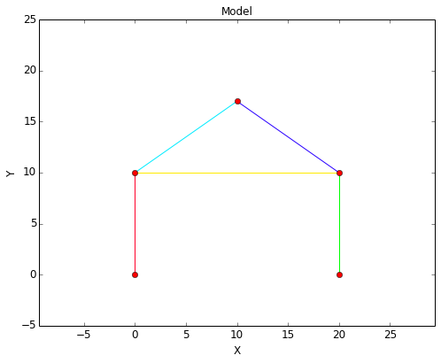
Every span connects 2 points and has a cross section and a material associated with it. In this case, a 1 inch circular cross section was specified along with Aluminum 6061-T6 material for each span in the model.

Materials and cross sections are specified in separate sections of this site, and once they are specified they can be used in the FEA model.

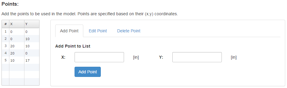
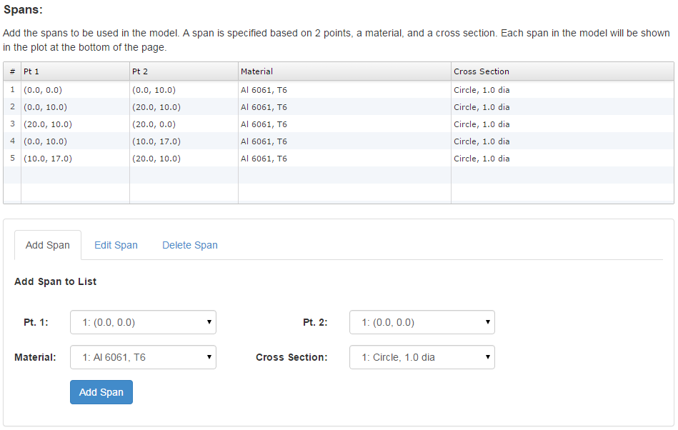
The inputs required to build this model are shown below. All of the points in the model are first specified, then the spans are specified by selecting 2 points as well as a material and a cross section for the span.

Applying Forces and Constraints

Once the geometry and materials are specified, the next step is to apply forces and constraints.

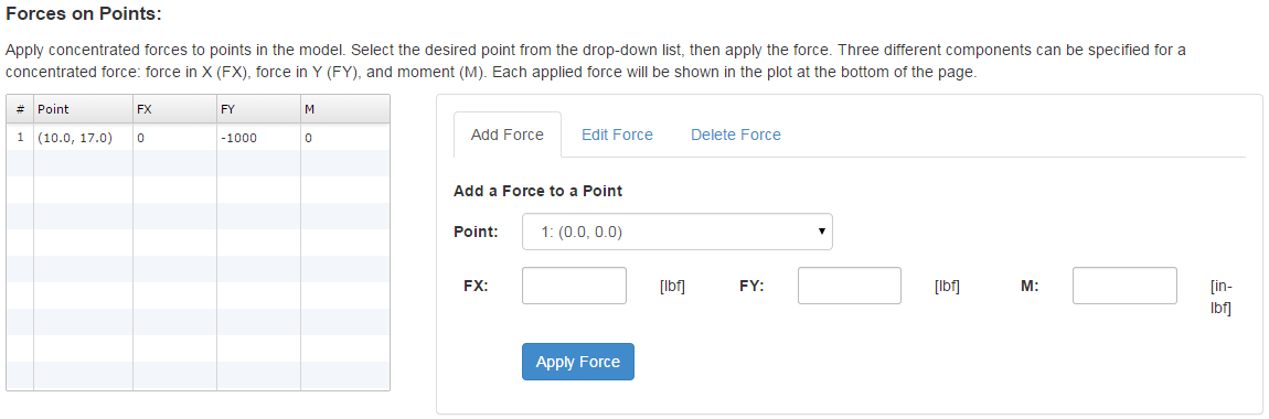
Concentrated Forces

Concentrated forces are applied to a specific point. Three different components can be specified for a concentrated force: force in X (FX), force in Y (FY), and moment (M).

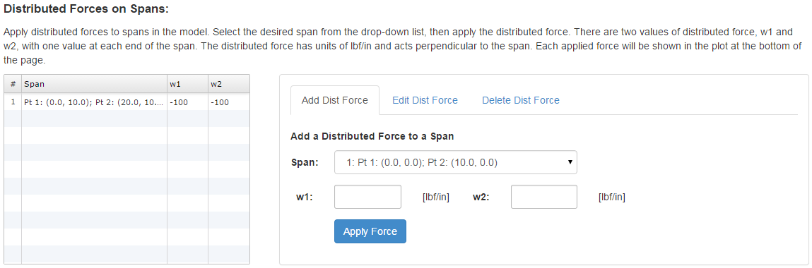
Distributed Forces

Distributed forces are applied over a span. There are two values of distributed force, w1 and w2, with one value at each end of the span. The distributed force has units of lbf/in and acts perpendicular to the span.

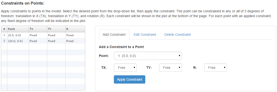
Constraints

Constraints are applied to a specific point. The point can be constrained in any or all of 3 degrees of freedom: translation in X (TX), translation in Y (TY), and rotation (R). For each point with an applied constraint, the constraint will be indicated in the model plot via text with the fixed degrees of freedom specified.

Common boundary conditions can be applied by specifying different combinations of constraints, as seen in the table below. The text that would be displayed on the model plot for each of these constraints is also given in the table for reference.

Boundary Condition	TX	TY	R	Display Text
Fixed	Fixed	Fixed	Fixed	X Y R
Pinned	Fixed	Fixed	Free	X Y
Guided in X	Free	Fixed	Fixed	Y R
Guided in Y	Fixed	Free	Fixed	X R
Roller in X	Free	Fixed	Free	Y
Roller in Y	Fixed	Free	Free	X

Forces and Constraints on Current Model

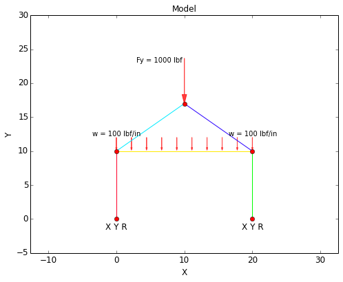
In this model, a concentrated force of 1000 lbf will be aplied to the point at the peak of the frame in the (-)Y direction, and a distributed force of 100 lbf/in will be applied along the cross bar in the (-)Y direction. Note that in the model, the concentrated force was applied to a point, whereas the distributed force was applied to a span.

The points at the base of each leg will be fixed in all degrees of freedom. Note that in the model plot below, the constraints on the points at the base of the frame are indicated by the text "X Y R."

The inputs required to specify the forces and constraints on this model are shown below:

Meshing and Solving

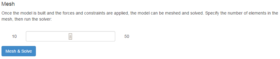
Once the model is built and the forces and constraints are applied, the model can be meshed and solved. The mesh for the current example is shown below. In the mesh plot, the element numbers are labeled.

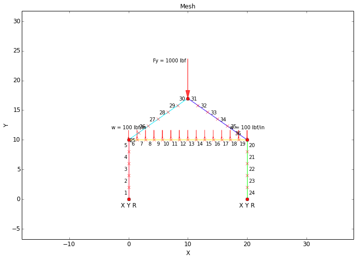
All that is required to mesh the model is to specify the number of elements in the mesh:

Viewing Results

There are a number of different results that are given as an output. These results include:

• Overview Plots
• Shear-Moment Diagram
• Stress Plots
• Displacement Plots
• Result Tables

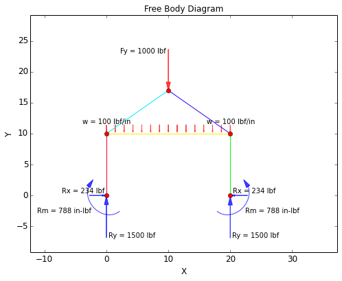
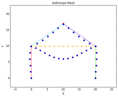
Overview Plots

In the 'Overview' section, the Free Body Diagram (FBD) is given that shows the applied forces and the reaction forces on the structure. The deformed mesh is also given that shows the node displacements on an exaggerated scale. The scale for the deformed mesh is automatically chosen for optimal viewing.

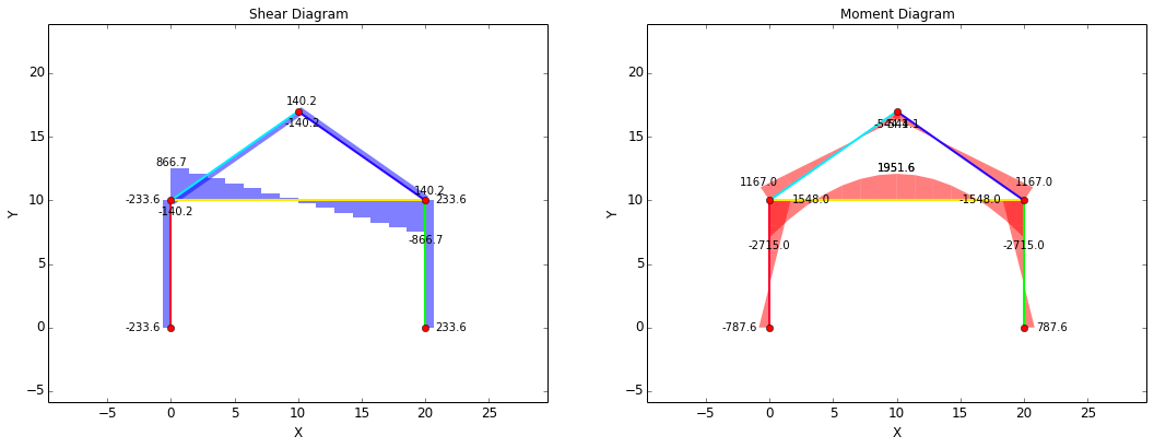
Shear-Moment Diagrams

The shear and moment diagrams for the current example are shown below. The standard sign conventions for shear-moment diagrams are followed:

• Shear: Positive shear causes clockwise rotation of the beam, negative shear causes counter-clockwise rotation.
• Moment: Positive moment will compress the top of the beam and elongate the bottom of the beam (i.e. make the beam 'smile').

Stress Plots

The stress plots for the current example are shown below.

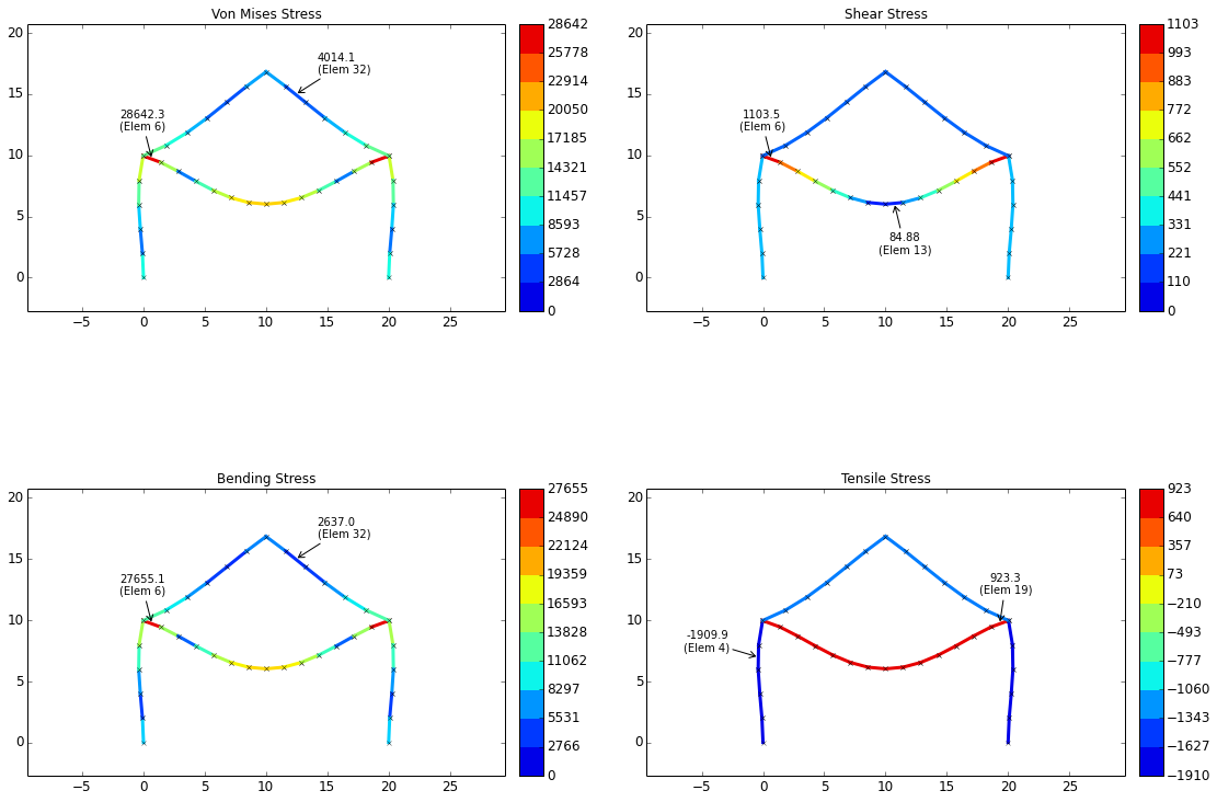
The stresses are calculated based on the equations below:

Axial Stress	Shear Stress	Bending Stress	Von Mises Stress
$$ \sigma_{ax} = {F_{ax} \over A} $$	$$ \tau_{sh} = {F_{sh} \over A} $$	$$ \sigma_{b} = {Mc \over I} $$	$$ \sigma_{vm} = \sqrt{ (\sigma_{ax} + \sigma_{b})^2 + 3\tau_{sh}^2 } $$

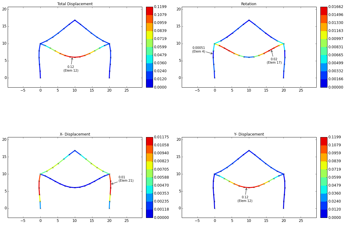
Displacement Plots

The displacement plots for the current example are shown below. The sign convention for displacements is:

• X: Positive to right, negative to left
• Y: Positive up, negative down
• Rotation: Right hand rule (positive counterclockwise, negative clockwise)

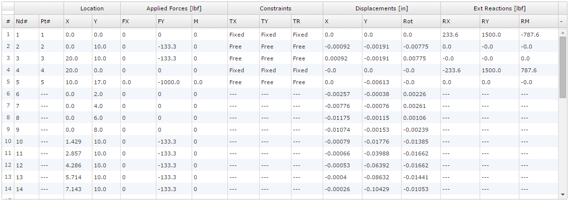
Result Tables

Result tables are given for nodal results and for elemental results.

The nodal result table for this example is shown below. This table shows the node numbers along with any associated point numbers (a node is created for every point in the model). The applied forces and constraints are shown on each node, where applicable, as well as the displacements and external reactions on each node. Note that external reactions will only be non-zero where constraints are applied.

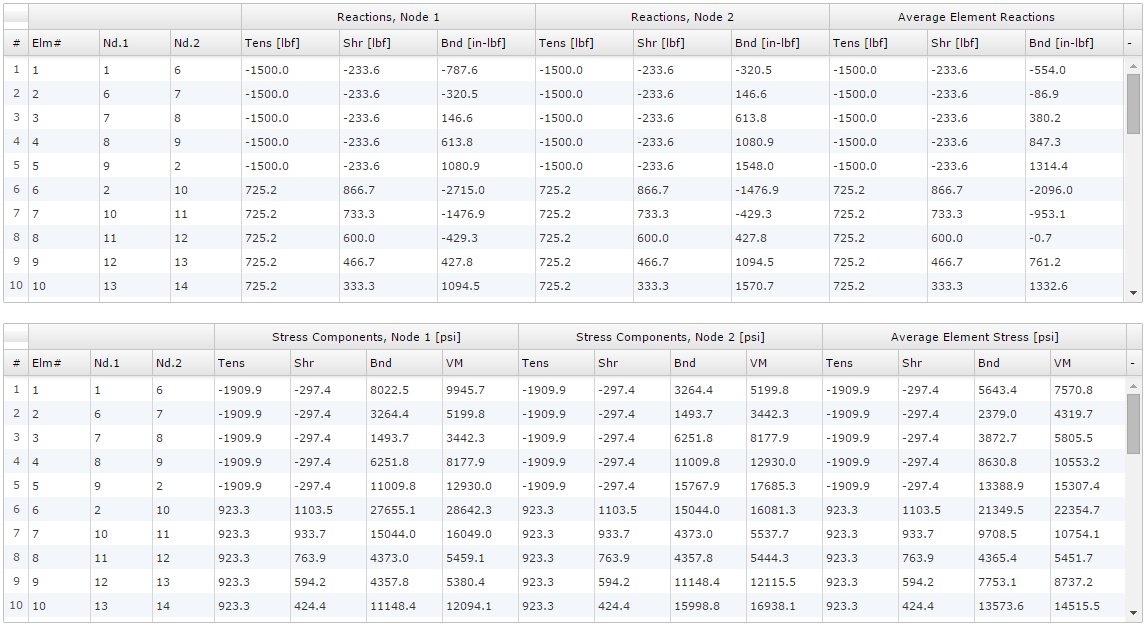
The elemental result tables for this example are shown below. Every element consists of two nodes; these nodes are referred to as "Node 1" and "Node 2" in the result tables. For example, in the first row of the table below it can be seen that Element 1 contains Node 1 and Node 6 in the mesh. For Element 1, "Node 1" refers to Node 1 and "Node 2" refers to Node 6.

In the first of the elemental result tables, the axial force, shear force, and bending moments are given for each node of each element. The average elemental forces are also given, which are simply the average of the nodal forces.

In the second of the elemental result tables, the axial, shear, bending, and von Mises stresses are given for each node of each element. The average elemental stresses are also given, which are simply the average of the nodal stresses.