


Strength of Materials
Strength of materials, also know as mechanics of materials, is focused on analyzing stresses and deflections in materials under load. Knowledge of stresses and deflections allows for the safe design of structures that are capable of supporting their intended loads.
Stress & Strain
When a force is applied to a structural member, that member will develop both stress and strain as a result of the force. Stress is the force carried by the member per unit area, and typical units are lbf/in2 (psi) for US Customary units and N/m2 (Pa) for SI units:

where F is the applied force and A is the cross-sectional area over which the force acts. The applied force will cause the structural member to deform by some length, in proportion to its stiffness. Strain is the ratio of the deformation to the original length of the part:

where L is the deformed length, L0 is the original undeformed length, and δ is the deformation (the difference between the two).
There are different types of loading which result in different types of stress, as outlined in the table below:
| Loading Type | Stress Type | Illustration |
|---|---|---|
| Axial Force |
|

|
| Shear Force | Transverse Shear Stress |

|
| Bending Moment | Bending Stress |

|
| Torsion | Torsional Stress |

|
Axial stress and bending stress are both forms of normal stress, σ, since the direction of the force is normal to the area resisting the force. Transverse shear stress and torsional stress are both forms of shear stress, τ, since the direction of the force is parallel to the area resisting the force.
| Normal Stress | |
|---|---|
| Axial Stress: |
|
| Bending Stress: |

|
| Shear Stress | |
|---|---|
| Transverse Stress: |

|
| Torsional Stress: |

|
In the equations for axial stress and transverse shear stress, F is the force and A is the cross-sectional area of the member. In the equation for bending stress, M is the bending moment, y is the distance between the centroidal axis and the outer surface, and Ic is the centroidal moment of inertia of the cross section about the appropriate axis. In the equation for torsional stress, T is the torsion, r is the radius, and J is the polar moment of inertia of the cross section.
In the case of axial stress over a straight section, the stress is distributed uniformly over the entire area. In the case of shear stress, the distribution is maximum at the center of the cross section; however, the average stress is given by τ = F/A, and this average shear stress is commonly used in stress calculations. More discussion can be found in the section on shear stresses in beams. In the case of bending stress and torsional stress, the maximum stress occurs at the outer surface. More discussion can be found in the section on bending stresses in beams.
We have a number of structural calculators to choose from. Here are just a few:

Just as the primary types of stress are normal and shear stress, the primary types of strain are normal strain and shear strain. In the case of normal strain, the deformation is normal to the area carrying the force:

|

|
In the case of transverse shear strain, the deformation is parallel to the area carrying the force:

|

|
where γ is the shear strain (unitless) and ϕ is the deformed angle in units of radians.
In the case of torsional strain, the member twists by an angle, ϕ, about its axis. The maximum shear strain occurs on the outer surface. In the case of a round bar, the maximum shear strain is given by:

|

|
where ϕ is the angle of twist, r is the radius of the bar and L is the length.
The shear strains are proportional through the interior of the bar, and are related to the max shear strain at the surface by:

where ρ is the radial distance from the bar's axis.
Hooke's Law
Stress is proportional to strain in the elastic region of the material's stress-strain curve (below the proportionality limit, where the curve is linear).

Normal stress and strain are related by:
where E is the elastic modulus of the material, σ is the normal stress, and ϵ is the normal strain.
Shear stress and strain are related by:
where G is the shear modulus of the material, τ is the shear stress, and γ is the shear strain. The elastic modulus and the shear modulus are related by:

where ν is Poisson's ratio.
Hooke's law is analogous to the spring force equation, F = k δ. Essentially, everything can be treated as a spring. Hooke's Law can be rearranged to give the deformation (elongation) in the material:
| Axial Elongation (from normal stress) |

|
|
| Angle of Twist (from shear/torsional stress) |

|
|
Strain Energy
When force is applied to a structural member, that member deforms and stores potential energy, just like a spring. The strain energy (i.e. the amount of potential energy stored due to the deformation) is equal to the work expended in deforming the member. The total strain energy corresponds to the area under the load deflection curve, and has units of in-lbf in US Customary units and N-m in SI units. The elastic strain energy can be recovered, so if the deformation remains within the elastic limit, then all of the strain energy can be recovered.

Strain energy is calculated as:
| General Form: | U = Work = ∫ F dL | (area under load-deflection curve) |
| Within Elastic Limit: |

|
(area under load-deflection curve) |

|
(spring potential energy) |
Note that there are two equations for strain energy within the elastic limit. The first equation is based on the area under the load deflection curve. The second equation is based on the equation for the potential energy stored in a spring. Both equations give the same result, they are just derived somewhat differently.
More information on strain energy can be found here.
We have a number of structural calculators to choose from. Here are just a few:
Stiffness
Stiffness, commonly referred to as the spring constant, is the force required to deform a structural member by a unit length. All structures can be treated as collections of springs, and the forces and deformations in the structure are related by the spring equation:
where k is the stiffness, F is the applied force, and δmax is the maximum deflection deflection in the member.
If the deflection is known, then the stiffness of the member can be found by solving k = F/δmax. However, the maximum deflection is typically not known, and so the stiffness must be calculated by other means. Beam deflection tables can be used for common cases. The two most useful stiffness equations to know are those for a beam with an axially applied load, and for a cantilever beam with an end load. Note that stiffness is a function of the material's elastic modulus, E, the geometry of the part, and the loading configuration.
| Stiffness [lbf/in] |
Max Deflection [in] |
Illustration | |
|---|---|---|---|
| Beam with axially applied load: |

|

|

|
| Cantilever beam with end load: |

|

|

|
The torsional equivalent of the of the spring equation is:
The stiffness of a shaft under torsional load is of particular interest:
| Stiffness [in*lbf/rad] |
Max Deflection [rad] |
Illustration | |
|---|---|---|---|
| Shaft with torsional load: |

|

|

|
Structure with Multiple Load Paths
If there are multiple load paths in a structure (i.e. there are multiple members in a structure that share the load), the load will be higher in the stiffer members. To find the load carried by any individual member, first calculate the equivalent stiffness of the members in the load path, treating them as springs. Depending on their configuration, they will be treated as some combination of springs in series and springs in parallel.
| Springs in Parallel | Springs in Series | |||
|---|---|---|---|---|
| Illustration: |

|

|
||
| Equivalent Stiffness of Structure: | keq = k1 + k2 + k3 + ... |

|
||
| Force in Individual Member: |
|
F1 = keqδtot = Fapp | ||
| Deflection in Individual Member: |

|
|
||
| Total Force in Structure: | Ftot = F1 + F2 + F3 + ... | Ftot = F1 = F2 = F3 = ... | ||
| Total Deflection in Structure: | δtot = δ1 = δ2 = δ3 = ... | δtot = δ1 + δ2 + δ3 + ... |


If the members in the load path cannot be treated purely as springs in series or as springs in parallel, but are rather a combination of springs in series and in parallel, then the problem will need to be solved iteratively. Find a sub-grouping of the members that are either purely in series or in parallel, and use the equations provided to calculate the equivalent stiffness, force and deflection in the sub-group. The sub-group can then be considered a single spring with the calculated stiffness, force, and deflection, and that spring can then be considered as a part of another sub-group of springs. Continue grouping members and solving until the desired result is achieved.
Stress Concentrations
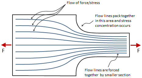
Forces and stresses can be thought to flow through a material, as shown in the figure below. When the geometry of the material changes, the flow lines move closer together or farther apart to accommodate. If there is a discontinuity in the material such as a hole or a notch, the stress must flow around the discontinuity, and the flow lines will pack together in the vicinity of that discontinuity. This sudden packing together of the flow lines causes the stress to spike up -- this peak stress is called a stress concentration. The feature that causes the stress concentration is called a stress riser.
Check out our interactive plots for common stress concentration factors.
Stress concentrations are accounted for by stress concentration factors. To find the actual stress in the viscinity of a discontinuity, calculate the nominal stress in that area and then scale it up by the appropriate stress concentration factor:
where σmax is the actual (scaled) stress, σnom is the nominal stress, and K is the stress concentration factor. When calculating the nominal stress, use the maximum value of stress in that area. For example, in the figure above, the smallest area at the base of the fillet should be used.
Many reference handbooks contain tables and curves of stress concentration factors for various geometries. Two of the most comprehensive collections of stress concentration factors are Peterson's Stress Concentration Factors and Roark's Formulas for Stress and Strain. MechaniCalc also provides a collection of interactive plots for common stress concentration factors.
The concentration of stress will dissipate as we move away from the stress riser. Saint-Venant's principle is a general rule of thumb stating that the distance over which the stress concentration dissipates is equal to the largest dimension of the cross section carrying the load.
Calculation of stress concentration is particularly important when the materials are very brittle, or when there is only a single load path. In ductile materials, local yielding will allow for stresses to be redistributed and will reduce the stress around the riser. For this reason, stress concentration factors are not typically applied to structural members made of ductile materials. Stress concentration factors are also not typically applied when there is a redundant load path, in which case yielding of one member will allow for redistribution of forces to the members on the other load paths. An example of this is a pattern of bolts. If one bolt starts to give, then the other bolts in the pattern will take more of the load.
Combined Stresses
At any point in a loaded material, a general state of stress can be described by three normal stresses (one in each direction) and six shear stresses (two in each direction):

The subscripts on the normal stresses, σ, indicate the direction of the normal stress. The subscripts of the shear stresses, τ, have two components. The first indicates the direction of the surface normal, and the second indicates the direction of the shear stress itself.
Commonly, the stresses along one direction are zero so that the full state of stress occurs on a single plane, as shown in the figure below. This is called plane stress. Plane stress occurs in thin plates, but it also occurs on the surface of any loaded structure. Surface stresses are commonly the most critical stresses since bending stress and torsional stress are maximized at the surface.

In the figure above, σx and σy are the normal stresses, and τ is the shear stress. The stresses balance so that the point is in static equilibrium. Because the shear stresses are all equal in magnitude, the subscripts are dropped for simplicity. (Note however that the sign of the stresses on the x face will be opposite to those on the y face.)
The proper sign conventions are as shown in the figure. For normal stress, tensile stress is positive and compressive stress is negative. For shear stress, clockwise is positive and counterclockwise is negative.
If the stresses from the figure above are known, it is possible to find the normal and shear stress on a plane rotated at some angle, θ, with respect to the horizontal, as shown in the figure below. The transformation equations below give the values of the normal stress and shear stress on this rotated plane.
| Normal Stress: |

|
| Shear Stress: |

|

Note that in the figure above, θ is measured from the x-axis, and a positive value of θ is counterclockwise.
At any point in the material, it is possible to find the angles of the plane at which the normal stresses and the shear stresses are maximized and minimized. The maximium and minimum normal stresses are called principal stresses. The maximum and minimum shear stresses are called the extreme shear stresses. The angles of the principal stresses and the extreme shear stresses are found by taking the derivative of each transformation equation with respect to θ and finding the value of θ where the derivative is zero.
| Principal Stress Angles: |

|
| Extreme Shear Stress Angles: |

|
The angles above can be substituted back into the transformation equations to find the values of the principal stresses and the extreme shear stresses:
| Principal Stresses: |

|
| Extreme Shear Stresses: |

|
The angles at which the principal stresses occur are 90° apart. Principal stresses are always accompanied by zero shear stress. The angles at which the extreme shear stresses occur are 45° from the angles of the principal stresses. Extreme shear stresses are accompanied by two equal normal stresses of (σx + σy) / 2.
A couple useful relationships are:
| σ1 + σ2 = σx + σy | The sum of the normal stresses is constant. |

|
The maximum shear stress is half the difference of the principal stresses. |
Mohr's Circle
Mohr's circle is a way of visualizing the state of stress at a point on a loaded material. It gives an intuitive feel to the stress transformation equations, and shows how the stresses on an element change as a function of the rotation angle, θ. From Mohr's circle, it also becomes clear what are the principal stresses, the extreme shear stresses, and the angles at which thoses stresses occur. An example of Mohr's circle is shown in the figure below:
Check out our Mohr's Circle calculator based on the methodology described here.

To construct Mohr's circle, first locate the center of the circle by taking the average of the normal stresses:

Place points on the circle representing the stresses on the x and y faces of the stress element. The stresses on the x face will have the coordinates ( σx , −τ ), and the stresses on the y face will have the coordinates ( σy , τ ). Place points on the circle for the principal stresses. The maximum principal stress will have the coordinates ( σ1 , 0 ), and the minimum principal stress will have the coordinates ( σ2 , 0 ). Place points on the circle for the extreme shear stresses. The maximum extreme shear stress will have coordinates ( σc , τ1 ), and the minimum extreme shear stress will have coordinates ( σc , τ2 ).
All of the points will lie on the perimeter of the circle. The circle has a radius equal to the magnitude of the extreme shear stresses:

The state of stress on the x and y faces of the stress element is represented by the black line in Mohr's circle connecting the points ( σx , −τ ) and ( σy , τ ). This line in Mohr's circle corresponds to the unrotated element in the figure below. If this line is rotated by some angle, then the values of the points at the end of the rotated line will give the values of stress on the x and y faces of the rotated element. It is important to note that the 360 degrees of Mohr's circle are equivalent to 180 degrees on the stress element. For instance, the points for x face and the y face are 180 degrees apart on Mohr's circle, but they are only 90 degrees apart on the stress element.

To get a more intuitive feel for how Mohr's circle relates the stresses on a stress element and how the stress state changes as a function of rotation angle, see the accompanying Mohr's circle calculator.
Applications
There are many structural components that are commonly subjected to stress analysis. The details on the analysis of these components are given in other sections:
We have a number of structural calculators to choose from. Here are just a few:
Allowable Stress Design
Knowledge of stresses and deflections allows for the safe design of structures that are capable of supporting their intended loads. It is always desired for the stresses in a structure to remain within the limits of the structure's strength. The yield strength of the material is commonly chosen as the strength limit to which the calculated stresses are compared.
The factor of safety, FS, is calculated as:

where σactual is the calculated stress in the structure, and σlimit is a maximum stress limit, typically a material strength such as the yield strength (Sty). The factor of safety indicates how far the actual stress is below the limiting stress. The FS value must be greater than or equal to 1 for the structure not to fail, but engineers will almost always design to some required factor of safety greater than 1. The required factor of safety will vary based on the criticality of the structure (i.e. the consequences if the structure were to fail) as well as the loading conditions (i.e. what types of loads are applied, how predictable are the loads, etc.). A high FS will result in a very safe structure, but if the value of FS is too high then the structure may become so large and heavy that it can no longer successfully perform its intended function. There are therefore many tradeoffs when selecting an appropriate factor of safety. Typical values of FS range from 1.15 to as high as 10.
The margin of safety is calculated as:

In the equation above, any value above zero indicates that the actual stress is below the limit stress. Although margins of safety are typically reported as decimal values, it is much more intuitive to think of margins as percentages. For example, if the limiting stress of a structure is 1.5 times higher than the actual stress, there is 50% margin (MS = 0.5).
When reporting factors of safety and margins of safety, sometimes the required factor of safety will be "baked in" to the reported factors. For example, the engineers may require a structure to maintain a factor of safety of at least 2, so that FSreq = 2. To bake in the required factor of safety, the reported FS and MS are calculated as:


Note that when including the required factor of safety, FSreq, the reported FS and MS are actually the margins with respect to FSreq, not with respect to the stress.
PDH Classroom offers a continuing education course based on this strength of materials reference page. This course can be used to fulfill PDH credit requirements for maintaining your PE license.
Now that you've read this reference page, earn credit for it!

References
- Budynas-Nisbett, "Shigley's Mechanical Engineering Design," 8th Edition
- Dowling, Norman E., "Mechanical Behavior of Materials: Engineering Methods for Deformation, Fracture, and Fatigue," 3rd Edition
- Gere, James M., "Mechanics of Materials," 6th Edition
- Lindeburg, Michael R., "Mechanical Engineering Reference Manual for the PE Exam," 13th Edition
- Pilkey, Walter D. and Pilkey, Deborah F., "Peterson's Stress Concentration Factors," 3rd Edition
- "Roark's Formulas for Stress and Strain," 8th Edition


