The theory of Finite Element Analysis (FEA) essentially involves solving the spring equation, F = kδ, at a large scale.

There are several basic steps in the finite element method:

1. Discretize the structure into elements. These elements are connected to one another via nodes.
2. Determine a local stiffness matrix for each element.
3. Assemble a global stiffness matrix for the overall structure based on the combination of the local stiffness matrices.
4. Build the applied force vector.
5. Apply boundary conditions and solve for the nodal displacements.
6. Solve for the external reactions.
7. Solve for nodal forces.
8. Solve for stresses.

In the first step, a mathematical model of the structure is composed. This model is an approximation of the structure -- whereas the physical structure is continuous, the model consists of discrete elements.

This analysis uses beam elements which are based on Euler-Bernoulli beam theory. The element has 2 nodes, each of which has 3 degrees of freedom: translation in x, translation in y, and rotation. A figure illustrating this element is shown below:

The element stiffness matrix for an Euler-Bernoulli beam element is shown below. This matrix represents the stiffness of each node in the element in a specific degree of freedom (i.e. it determines the displacement of each node in each degree of freedom under a given load). Because each of the nodes in the beam element have 3 degrees of freedom, a 6 x 6 matrix can completely describe the stiffness of the element.

The global stiffness matrix for the overall structure is assembled based on the combination of the local stiffness matrices. At a high level, the global stiffness matrix is created by summing the local stiffness matrices:

where the matrix [k_i] is the local stiffness matrix of the i^th element.

The global stiffness matrix will be a square n x n matrix, where n is 3 times the number of nodes in the mesh (since each node has 3 degrees of freedom). When assembling the global stiffness matrix, the stiffness terms for each node in the elemental stiffness matrix are positioned in the corresponding location in the global matrix. For any elements which share a node, the stiffness contributions of that node will be summed from each element.

The applied force vector will be an n x 1 vector, where n is 3 times the number of nodes in the mesh. The force vector is assembled by including the applied forces on each degree of freedom on each node in the mesh:

Once the global stiffness matrix and the applied force vector are built, the nodal displacements can be solved for. The following equation relates the forces and displacements in the overall structure:

where {F} is the applied force vector, {R} is the external reaction vector, [K] is the global stiffness matrix, and {U} is the nodal displacement vector.

In the equation above, {R} and {U} are unknowns. To simplify the solution of this equation, it is desired to solve for the reactions and displacements independently of one another. To do this, we can use the fact that for every constraint that was applied (either a constraint in x-translation, y-translation, or rotation), the displacement associated with that constraint will be zero. Additionally, external reactions will only occur where constraints were applied. Therefore, it is known that for every degree of freedom on every node:

• If a constraint is applied, displacement at that constraint will be zero, and the external reaction may be non-zero.
• If there is no constraint, the external reaction will be zero, and the displacement may be non-zero.

We will initially solve the equation above for nodal displacements, {U}. Based on the reasoning above, it is possible to remove the {R} vector from the equation. Boundary conditions are applied to the equation by "zeroing out" the rows in the matrices corresponding to applied constraints. By doing this, we haven't lost any information about the nodal displacements since it is known that the displacements will be zero for each row that was zeroed out. Now the equation has reduced to:

The equation above can be solved for {U}, after which all of the nodal displacements are known. The only unknown remaining in the original equation is {R}, and this can now be solved for:

It is now possible to solve for the forces on each node. For any reaction force that was found, the nodal force is just equal to the reaction force. However, for any nodes where there is no external reaction, the forces on the node are still unknown. These can be found by extracting the appropriate displacements from the global {U} vector to build a local {u} vector for each element. Each of these local vectors will be a 6 x 1. The nodal forces on each element can be solved using:

where {f } is the element (local) force vector, [k] is the element stiffness matrix, and {u} is the element displacement vector.

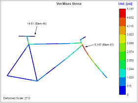
Once the forces are known on each node in the mesh, it is possible to solve for stresses at each node:

Axial Stress	Shear Stress	Bending Stress	Von Mises Stress

---

---

References

1. Moaveni, Saeed, "Finite Element Analysis Theory and Application with ANSYS," 2nd Ed.