This page describes selected topics in algebra that are of particular importance in mechanical engineering.

Linear Interpolation

Linear interpolation is the process of finding a point that lies on a line between two other points. This is particularly useful when you have a set of data and need to approximate values between the data points.

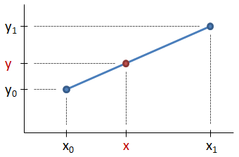
Assume that you have two data points, ( x₀ , y₀) and ( x₁ , y₁), as shown in the figure below. You need to find the point ( x , y), highlighted in red in the figure, which lies between the two points. You know the value of x and want to find the corresponding value of y.

Since the slope of the line from ( x₀ , y₀) to ( x , y) is the same as the slope of the line from ( x₀ , y₀) to ( x₁ , y₁), it follows that:

Solving for y, we have the interpolation equation:

Alternate Interpolation Method

A helpful trick is to recognize that the proportion of x between x₀ and x₁ is the same as the proportion of y between y₀ and y₁. For example, if x is 25% of the way between x₀ and x₁, then y is also 25% of the way between y₀ and y₁.

Therefore, a procedure for interpolating without having to remember the interpolation equation is as follows:

• Find the proportion of x between x₀ and x₁:

  

• Note that p_y, the proportion of y between y₀ and y₁, is equal to the value of p_x calculated above:
  p_y = p_x
• Write the formula for the proportion of y between y₀ and y₁, and solve for y:

  ⟹

Note that this process still yields the interpolation equation, it's just a slightly different way of approaching the problem.

---

---

Normalizing a Data Set

Normalization is the process of scaling a set of data such that the sum of the resulting data set is equal to 1. This is accomplished by summing each value in the data set, and then the normalized value for each of the values in the data set is calculated by dividing it by the sum:

where in the equation above, n_i is the normalized value of the i^th term in the data set, v_i is the i^th value, and Σ v is the sum of every term in the data set.

One use of normalization is to compare multiple data sets that have different scales (i.e. if you want to use a set of data that is composed of very large numbers alongside another set of data that is composed of very small numbers). The data sets can be normalized to remove the effect of the differing scales.

It should be noted that normalizing a data set is similar to normalizing a vector but with the key difference that when a vector is normalized each component of the vector is divided by the vector's magnitude rather than the sum of the terms.

Determining an Exponential Equation Given Two Points

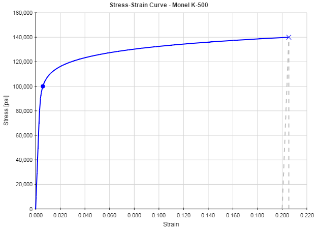
There are many phenomena in engineering that can be described by an exponential curve. Very frequently, two points along that curve will be known and it is desired to determine the equation for the curve knowing only those two points. For example, the plastic region of a material's stress-strain curve can be approximated by an exponential curve, and the yield point and the failure point for the material will commonly be known. With that information, an approximate equation for the stress-strain curve can be determined. Another example is the S-N curve for the fatigue life of a material.

An example of a stress-strain curve for the material Monel K-500 is shown below. If we know only the points on the curve corresponding to the yield strength and the ultimate strength, the entire stress-strain curve can be constructed.

An exponential equation is of the form:

where a and k are the constants of the equation. If two points along the exponential curve are known, then these constants can be determined by:

where, in the equations above, ( x₁ , y₁) and ( x₂ , y₂) correspond to two points on the curve.

To derive the equations above, it is important to realize that exponential equations, when converted to logarithmic, become linear (so that if you plot an exponential curve on a log-log plot, the curve is a straight line). Using the properties of logarithms, the exponential equation can be converted into logarithmic form:

y = axk

⟹

log(y) = k log(x)+ log(a)

On a logarithmic plot, the above logarithmic equation is equivalent to y = mx + b, where

y = log(y) ,

x = log(x) ,

m = k ,

b = log(a)

The unknowns above are the values for k and a. To determine k, we can calculate the slope of the logarithmic curve. For the linear equation, that would be done by:

The equivalent for the logarithmic equation is:

To determine the constant a, we calculate the intercept of the logarithmic curve. For a linear equation y = mx + b, the intercept is calculated as b = y₁ − m x₁, where ( x₁ , y₁) is a point on the line. For the logarithmic curve, the intercept is calculated as:

Note that the constant a can also be solved for directly using the original exponential equation once a value is found for k. Substituting values for the point ( x₁ , y₁) and solve for a:

⟹

Now that the constants have been found from the two points on the curve, the exponential equation is known.

---

---

References

1. Dowling, Norman E., "Mechanical Behavior of Materials: Engineering Methods for Deformation, Fracture, and Fatigue," 3rd Ed.
2. Kreyszig, Erwin, "Advanced Engineering Mathematics," 10th Ed.
3. Lindeburg, Michael R., "Mechanical Engineering Reference Manual for the PE Exam," 13th Ed.

---